3  Results

Data pre-processing

Code

# Data pre-processing for results and analysis
library(ggplot2)
library(dplyr)
library(scales)
library(forcats)
library(ggmap)
library(sf)
library(readxl)
library(tmap)
library(vcd)
library(lubridate)
library(viridis)

df <- read.csv("/Users/kaitlynbrown/Desktop/STAT5702/Rat_Sightings.csv")
df<- mutate(df, Created.Date = as.Date(Created.Date, format = "%m-%d-%Y"))
#"/Users/kaitlynbrown/Desktop/STAT5702/Rat_Sightings.csv"
df$Year <- year(df$Created.Date)
#df2: used for rat sightings per day by borugh
df2 <- df[df$Borough != "Unspecified",]
df2 <- df2[df2$Borough != "",]

# List of location types in NYC
locations = list("3+ Family Mixed Use Building", "3+ Family Apt. Building", "1-2 Family Dwelling", "1-2 Family Mixed Use Building", "Commercial Building")

#df3 : used for rat sightings per day by borough
df3 <- df[df$Location.Type %in% locations,]


# Calling stadia map
register_stadiamaps('e51b7311-980d-4703-bc7d-9afa1014b3c1')
nyc_map <- get_stadiamap(bbox = c(left = -74.2591, bottom = 40.4774, 
                                 right = -73.7002, top = 40.9162),
                        zoom = 10, maptype = "stamen_toner_lite")

# Sampling the map
df_sample = sample_n(df, nrow(df)/10)

# Getting zipcode shape file
zipcodes = st_read("/Users/kaitlynbrown/Desktop/STAT5702/nyc.shp",quiet=TRUE)
# KB's file path : '/Users/kaitlynbrown/Desktop/STAT5702/nyc.shp'
# Making the zipcode shape 
zipcodes <- zipcodes %>% 
       rename(Incident.Zip = 'modzcta')

df4 <- df %>% group_by(Incident.Zip) %>% 
  summarise(total_count=n(),
            .groups = 'drop')

map_df <- left_join(zipcodes, df4)

# Create dataframe for summarizing for incident and location type
df5 <- df3 %>% group_by(Incident.Zip, Location.Type) %>% 
  summarise(total_count=n(),
            .groups = 'drop')

# Create dataframe grouped by location type
df6 <- df3 %>% group_by(Location.Type) %>% 
  summarise(total_count_loc=n(),
            .groups = 'drop')

# Left join summarized (incident and location type charts) with dataframe grouped by location type and add a total count column as a percentage of total location count
df5 <- left_join(df5,df6)
df5 <- df5[df5$Location.Type != "",]
df5$proportion <- df5$total_count / df5$total_count_loc

# Create a dataframe by joining zipcodes with the combined (location type, %total counts,source mapped)
map_df2 <- left_join(zipcodes, df5)

# Creating a dataframe by grouping years together.
df7 <- mutate(df3, Year.Range = case_when(
    Created.Date < as.Date("01-01-2014", format = "%m-%d-%Y") ~ "2010-2013",
    Created.Date < as.Date("01-01-2018", format = "%m-%d-%Y") & Created.Date >= as.Date("01-01-2014", format = "%m-%d-%Y") ~ "2014-2017",
    Created.Date < as.Date("01-01-2022", format = "%m-%d-%Y") & Created.Date >= as.Date("01-01-2018", format = "%m-%d-%Y") ~ "2018-2021",
    Created.Date >= as.Date("01-01-2022", format = "%m-%d-%Y") ~ "2022-2023"
    ))

#Changing the name of the status of rat sighting actions in the dataframe
df7 <- mutate(df7, Status = case_when(
    Status == "Closed" ~ "Closed",
    Status == "Pending" ~ "Not Closed",
    Status == "Assigned" ~ "Not Closed",
    Status == "In Progress" ~ "Not Closed",
    Status == "Open" ~ "Not Closed",
    Status == "Unspecified" ~ "Not Closed"))

# Cleaning out the dataset with low % categories
df7 <- df7[df7$Borough != 'STATEN ISLAND',]
df7 <- df7[df7$Borough != 'Unspecified',]
df7 <- df7[df7$Location.Type != '3+ Family Mixed Use Building',]
df7 <- df7[df7$Location.Type != '1-2 Family Mixed Use Building',]

Question 1: How has the number of 311-reported rat sightings in NYC changed over time? How does this trend differ across different boroughs and location types?

Code

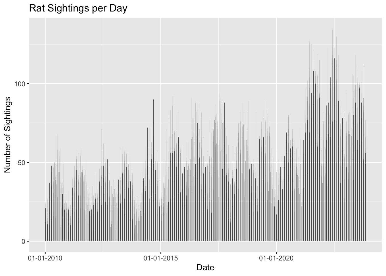
# Plot 1: Rat sightings per day
# Count sightings per year
ggplot(df, aes(Created.Date)) +
    geom_bar(stat="count", na.rm = TRUE) +
    ggtitle("Rat Sightings per Day") +
    xlab("Date") + ylab("Number of Sightings") +
    scale_x_date(labels=date_format ("%m-%d-%Y"))

We can see that there is a seasonal cycle in 311 requests for rat sightings. Sightings are lowest at the beginnings and ends of the year and peak mid-year. This indicates that rat sightings may be positively correlated with warmer temperatures. We can also see that rat sightings have increased overall over the past 13 years, with the sharpest increases in the mid 2010s and in 2021 and 2022.

Code

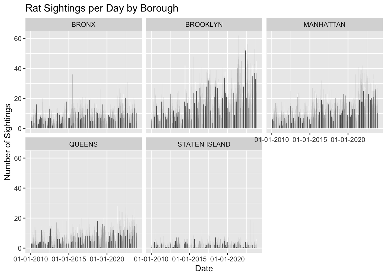
ggplot(df2, aes(Created.Date)) +
    geom_bar(stat="count", na.rm = TRUE) +
    ggtitle("Rat Sightings per Day by Borough") +
    xlab("Date") + ylab("Number of Sightings") +
    scale_x_date(labels=date_format ("%m-%d-%Y")) +
    facet_wrap(~Borough)

Faceting by borough, we see that the seasonal trend holds true across the boroughs. We can see differences in the overall trend across the boroughs. The Bronx, Queens, and Staten Island have generally seen an increase in sightings over the past 13 years. Brooklyn and Manhattan, however, have seen much sharper increases.

Code

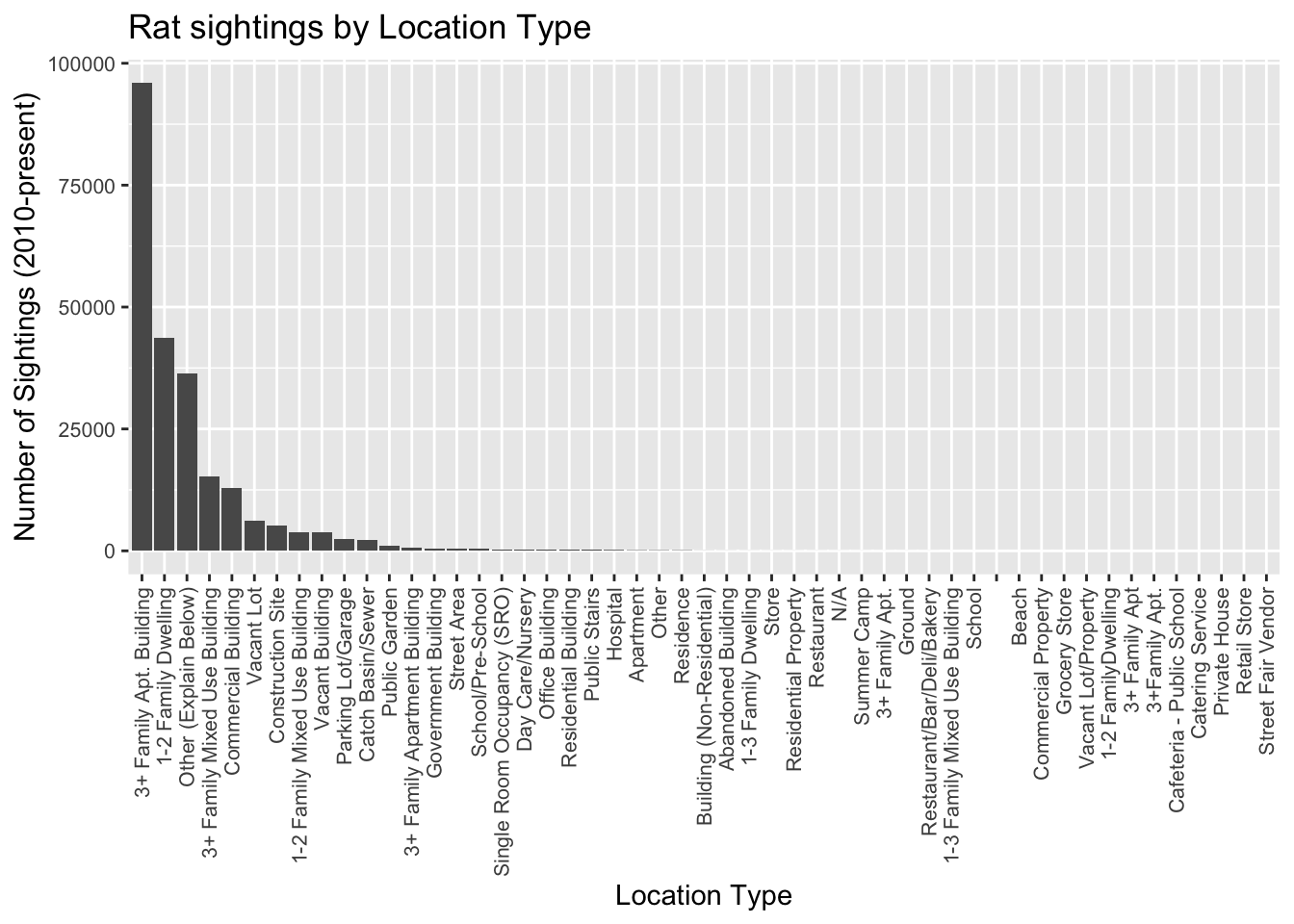
# Plot 5: Overall Rat sightings by location type
df_filtered <- df %>%
  group_by(Location.Type) %>%
  summarize(Count = n()) %>%
  filter(Count >= 10000) %>%
  right_join(df, by = "Location.Type")

# Plotting
ggplot(df_filtered, aes(fct_infreq(Location.Type))) +
    geom_bar(stat="count", na.rm = TRUE) +
    ggtitle("Rat sightings by Location Type")+
    xlab("Location Type") +  # Label for the x-axis
    ylab("Number of Sightings (2010-present)") +  # Label for the y-axis
    theme(
        axis.text.x = element_text(angle = 90, vjust = 0.5, hjust = 1, size = 8),  # Customize x-axis text
        axis.text.y = element_text(size = 8)  # Customize y-axis text
    )

We can see that the most common locations for rat sightings are 3+ family apartments, 1-2 family dwellings, 3+ family mixed use buildings, and commercial buildings. Of course, this is likely due to the fact that these location types are more prevalent in NYC than the other location types. We cannot conclude that rats are more likely to be sighted in these location types without information on the prevalence of these location types in NYC. However, this information is useful for the following analysis and knowing which location types to focus on.

Code

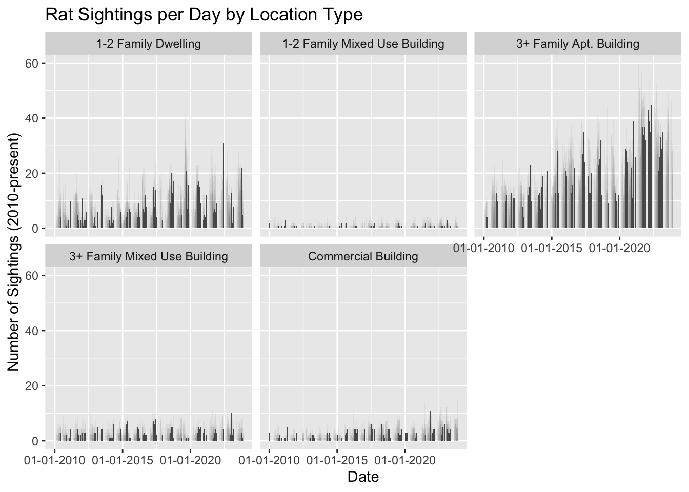
ggplot(df3, aes(Created.Date)) +
    geom_bar(stat="count", na.rm = TRUE) +
    ggtitle("Rat Sightings per Day by Location Type") +
    xlab("Date") + ylab("Number of Sightings (2010-present)") +
    scale_x_date(labels=date_format ("%m-%d-%Y")) +
    facet_wrap(~Location.Type)

We can see that there is one apparent difference in the trend of rat sightings over time for different location types. 3+ family apartment buildings do not have as strong of a seasonal trend as the other location types. This indicates that the change in temperature does not affect the presence of rats within apartment buildings as significantly as it does for businesses or homes. The overall trend is also a much sharper increase in sightings for 3+ family apartment buildings and commercial buildings than the other location types.

Question 2: Which regions of NYC have the most rat sightings? How does that change across location types?

Code

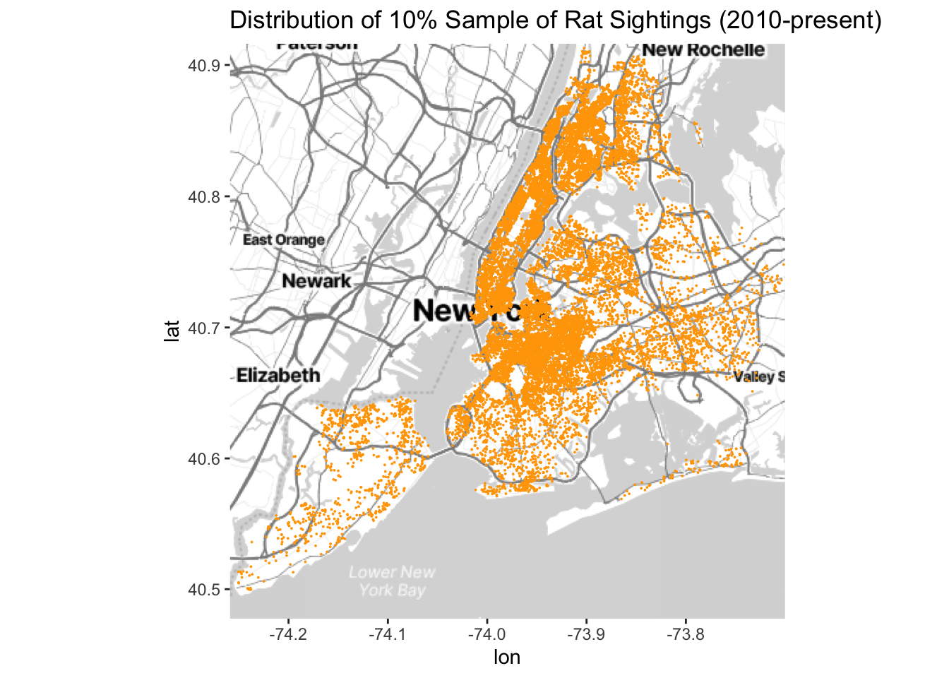
# Plot 2: Overall concentration of Rat Sightings so far on an NYC Map using geo-coordinates
library(ggmap)
ggmap(nyc_map) +
  geom_point(data = df_sample, aes(x=Longitude,y=Latitude), size = 0.005, color = 'orange')+
  ggtitle("Distribution of 10% Sample of Rat Sightings (2010-present)")

This plot shows a random sample of just 10% of all 311 requests for rat sightings across the city. We can see that sightings are most dense in Manhattan, upper Brooklyn, and the Bronx. Before affirmatively concluding that one is more likely to see rats in these areas, it is still important to consider the differences in the population density of these areas.

Code

library(tmap)

tmap_mode("view")
tm_shape(map_df) +
  tm_polygons("total_count", id = 'Incident Zip', palette = "viridis") +
  tm_bubbles(size = 0.05, popup.vars = c("Zip Code" = "Incident.Zip"))+
  tm_layout("Rat Sightings from 2010-2023 by Zip Code",
            title.size = 0.95, frame = FALSE)

This plot allows us to look at the location of rat sightings on a more specific scale by zip code. Here, one trend that could not be seen in the previous plot is apparent. The Upper West side, particularly the 10025 zip code, has many more rat sightings than the rest of Manhattan.

Code

library(tmap)
library(viridis)

# Setting tmap to interactive viewing mode
tmap_mode("view")

# Create the faceted plot without legends
tm_shape(map_df2) +
  tm_polygons("proportion", palette = "viridis", show.legend = FALSE) +
  tm_facets(by = "Location.Type")

We can also consider this plot faceted by the most common location types. The biggest noticeable difference here is that the zip codes in Brooklyn are the strongest hotspots for 1-2 family dwellings, 1-2 family mixed use buildings, and 3+ family apartment buildings. The Upper West Side hotspot is strongest for 3+ family apartment buildings and 3+ mixed use buildings. Again, it is important to consider the underlying distributions here and which location types are generally more common in these zip codes.

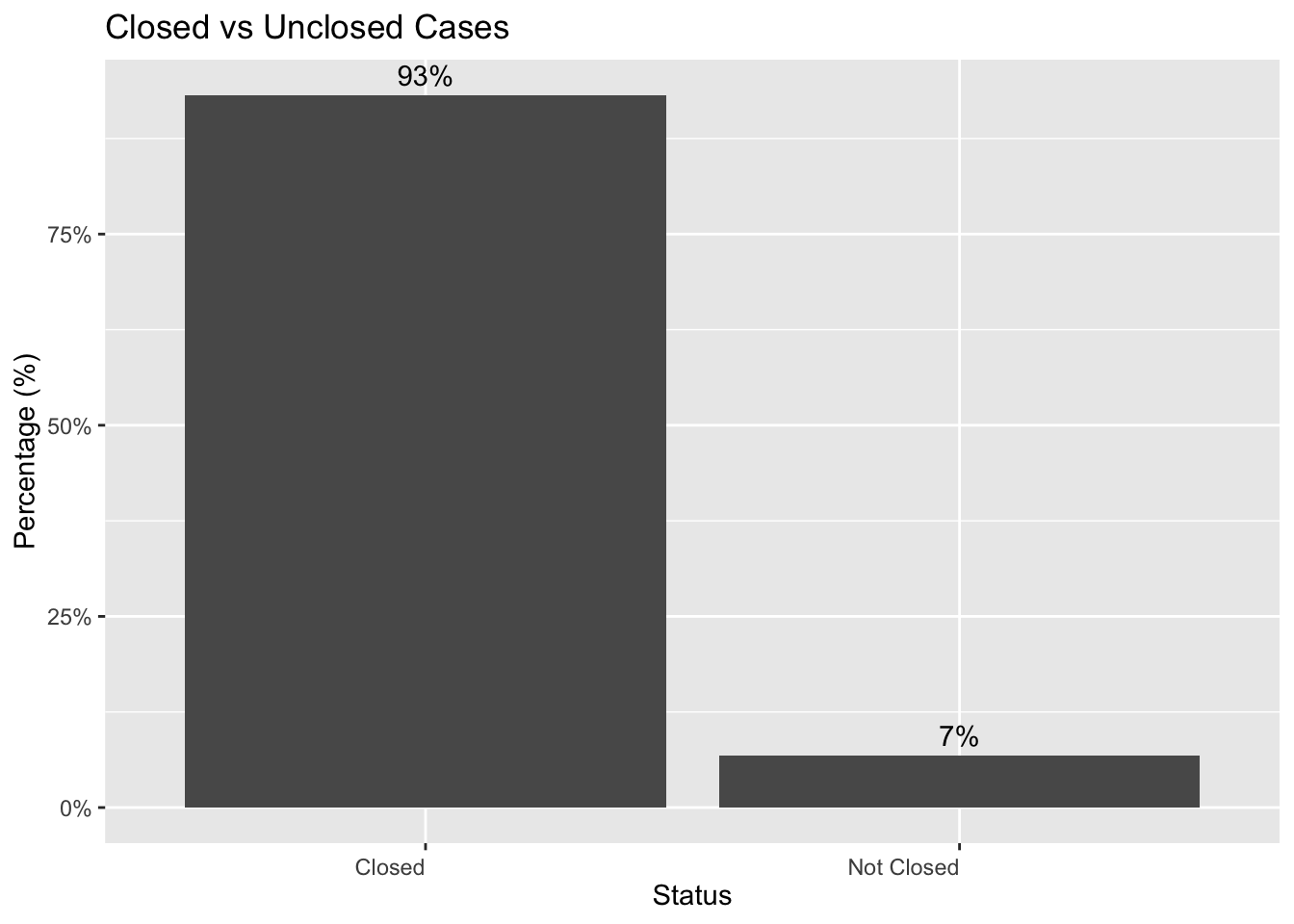
Question 3: What factors influence whether a 311 request for a rat sighting is marked as closed?

Code

# Plot 8
library(forcats)
library(scales)

total_count <- sum(table(df7$Status))

ggplot(df7, aes(x = fct_infreq(Status))) +
    geom_bar(aes(y = ..count.. / total_count * 100), stat="count", na.rm = TRUE) +
    geom_text(aes(label = scales::percent(..count.. / total_count, accuracy = 1),
                  y = ..count.. / total_count * 100), 
              stat="count", vjust = -0.5) +  # Add percentage labels
    ggtitle("Closed vs Unclosed Cases") +
    xlab("Status") +
    ylab("Percentage (%)") +
    scale_y_continuous(labels = scales::percent_format(scale = 1)) +
    theme(axis.text.x = element_text(angle = 0, vjust = 0.5, hjust=1))

Here, we can see that the vast majority of 311 requests for rat sightings in the past 13 years have been marked as closed. The remaining in the “not closed” category are primarily pending, in progress, or assigned.

Code

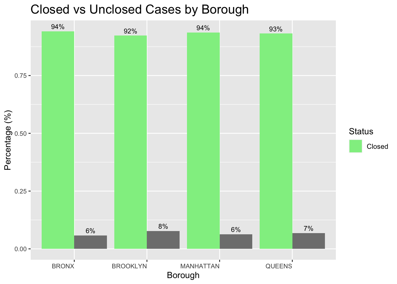
df7_grouped <- df7 %>%
  count(Borough, Status) %>%
  group_by(Borough) %>%
  mutate(Percent = n / sum(n))

# Create the plot
ggplot(df7_grouped, aes(x = Borough, y = Percent, fill = Status)) +
  geom_bar(stat = "identity", position = position_dodge()) +
  geom_text(aes(label = scales::percent(Percent, accuracy = 1)),
            position = position_dodge(width = 0.9), vjust = -0.5, size = 3) +
  ggtitle("Closed vs Unclosed Cases by Borough") +
  xlab("Borough") +
  ylab("Percentage (%)") +
  scale_fill_manual(values = c("Closed" = "lightgreen", "Pending" = "lightyellow")) +
  theme(
    axis.text.x = element_text(angle = 0, hjust = 1, size = 8),  
    axis.text.y = element_text(size = 8),  
    plot.title = element_text(size = 16)  
  )

This is true across boroughs.

Code

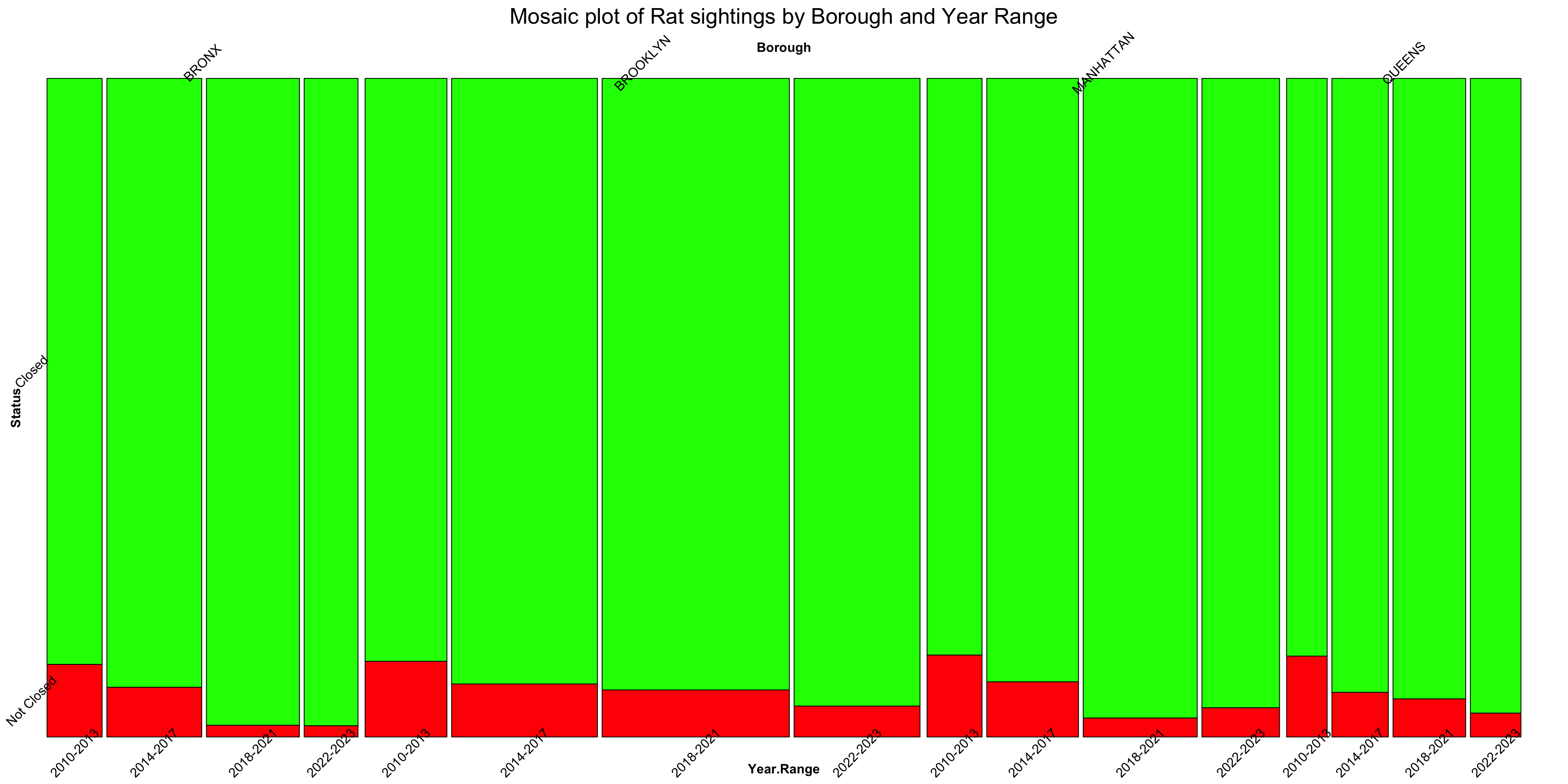
#Plot 9: Plotting a mosaic plot, using Borugh as a categoric feature
mosaic(Status ~ Borough + Year.Range, data = df7,
       direction = c('v', 'v', 'h'),
       main = 'Mosaic plot of Rat sightings by Borough and Year Range',
       highlighting_fill = c('green','red'), labeling = vcd::labeling_border(rot_labels = c(45, 45)))

We can consider whether the year the request was made is correlated with how likely it is to be marked as closed. We can also consider whether the borough the request was made for is correlated with how likely it is to be marked as closed. Staten Island has been excluded here due to low overall rat sightings. Generally, across all boroughs, the proportion of unclosed requests has consistently decreased over the years. There does not appear to be a correlation between borough and whether a request is closed.

Code

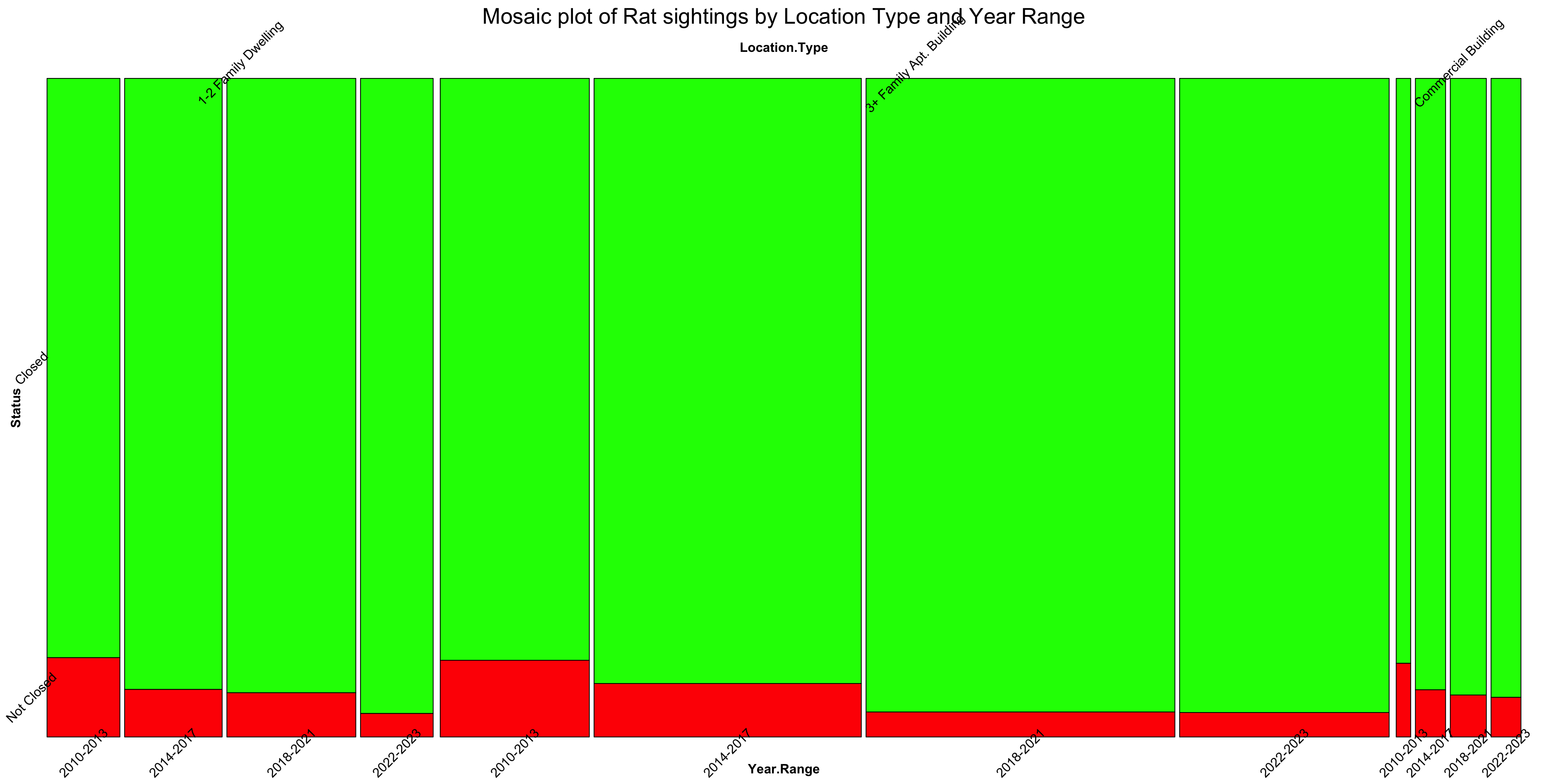
#Plot 10: Plotting a mosaic plot, using Location type as a categoric fearure
mosaic(Status ~ Location.Type + Year.Range, data = df7,
       direction = c('v', 'v', 'h'),
       main = 'Mosaic plot of Rat sightings by Location Type and Year Range',
       highlighting_fill = c('green','red'), labeling = vcd::labeling_border(rot_labels = c(45, 45)))

We can also see that there does not appear to be a correlation between location type and whether a request is closed. The trend of decreasing proportion of unclosed requests holds true across location types.